Text Classification for Flipkart Product Reviews
- hxr8557
- Nov 30, 2022
- 11 min read
Updated: Dec 1, 2022

Image source : flipkart-reviews
Introduction :
The main goal of this blog is to dive deep into various algorithms that can be used in the field of text classification, and compare their performance and accuracies with each other. Here, we will be considering the Product Review Dataset from Kaggle, which contains all the user given reviews for electronic products on Flipkart.
The main aim is to classify these reviews as positive/negative/neutral.
Acknowledgement :
I acknowledge that I followed the below tutorial to implement the text classification for product review data. On top of this existing model, I've done my experiment on hyper parameters tuning - to analyze how the models would behave with different hyper parameters. We will walk through that part, in the later section of this blog.
Links to my profile and notebook :
Link to my GitHub profile ( You can refer my Jupyter notebook here ): https://github.com/harshithaharshi/text_classification/blob/main/Final_Project_DM.ipynb
Jupyter Notebook uploaded in Kaggle :
Link to my YouTube Video ( A quick advertisement ) :
Dataset Description:
Dataset Name : Flipkart_Reviews - Electronics
(Note : The above dataset - was suggested in our Data Mining Final project instructions)
Download Link : https://www.kaggle.com/datasets/vivekgediya/ecommerce-product-review-data?select=Flipkart_Reviews+-+Electronics.csv
Description and Important features :
This dataset represents the product reviews given by the users in the Flipkart e-commerce platform. It contains the reviews in the form of text reviews, rating, upvotes, downvotes and summary. We will be mainly focusing on these features, to perform the classification on the reviews.

Image source : https://www.vecteezy.com
Overview of the different algorithms used :
Let's look into the different algorithms used in this implementation.
1 - Logistic Regression
2 - K-Nearest Neighbor (KNN)
3 - Support Vector Machine (SVM)
4 - Decision Trees (DT)
5 - Naive Bayes
Before getting started, let's look at the brief introduction of the above mentioned algorithms.
1 - Logistic Regression :
Logistic regression is an example of supervised learning. It is used to calculate or predict the probability of a binary (yes/no) event occurring. An example of logistic regression could be applying machine learning to determine if a person is likely to be infected with COVID-19 or not [11]
To use Logistic Regression for multi class classification - we use Sigmoid function to calculated the probabilities for each class.
2 - KNN :
KNN [12] works by finding the distances between a query and all the examples in the data, selecting the specified number examples (K) closest to the query, then votes for the most frequent label (in the case of classification) or averages the labels (in the case of regression).
3 - SVM :
SVM [13] or Support Vector Machine is a linear model for classification and regression problems. It can solve linear and non-linear problems and work well for many practical problems. The idea of SVM is simple: The algorithm creates a line or a hyperplane which separates the data into classes.
4 - Decision Tree :
A decision tree [14] is a non-parametric supervised learning algorithm, which is utilized for both classification and regression tasks. It has a hierarchical, tree structure, which consists of a root node, branches, internal nodes and leaf nodes.
5 - Naive Bayes :
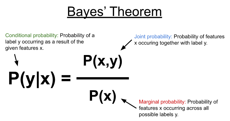
A Naive Bayes classifier [15] is a probabilistic machine learning model that’s used for classification task. The crux of the classifier is based on the Bayes theorem.
Code Implementation :
Now, let's go through the step by step code implementation of this existing model, that I have referred to. [1]
1 - Importing all the necessary libraries.
Basic libraries
NLTK libraries
Machine Learning libraries
Metrics libraries
Visualization libraries
And, other miscellaneous libraries

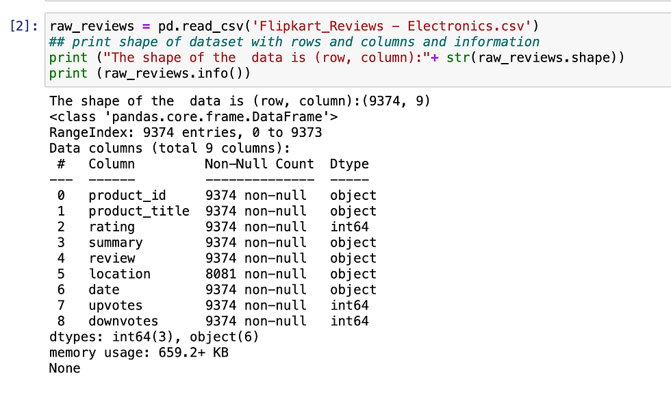
2 - Load the data from the given file.
In this step, we will load the review data from the given file. If we observe, our dataset has - 9373 rows and 9 columns. Below screenshot gives the detailed info about the dataset we will be using here.
3 - Data Pre-processing
As we know, Data preprocessing is a very important step before we get into the actual implementation. Here, we will check for NaN values. As a result, there's no NaN values present in the review and summary columns (these will be the prime review columns). So, we don't have to worry about null values!

4 - Merging the two review columns into one
In our data, we have two columns which convey the same objective i.e. review and summary column. Summary is a shorter version of the review, where as the review column gives a detailed description of the review. so, we can merge these two columns for our easy processing. Merging these two columns will not have any effect on the meaning of the reviews.


A sample review, after merging the two columns:

5 - Analyzing the sentiment of the reviews.
In this step, we will create the outcome column - which indicates the sentiment of a review. We make use of the rating to arrive at this decision.
If the rating is greater than 3, we take that as an positive sentiment and if the rating is less than 3 it is negative. If it is equal to 3, we take that as neutral sentiment
Taking the count of each category of ratings :

Function to determine the sentiment of a review, based on its rating

Applying the above function to derive our new outcome column - 'sentiment'

Now, we will be able to see the overall count of positive, negative and neutral reviews

6 - Text Pre-processing
Defining the function to process the review data. In this processing, we will aim at removing all the special characters, digits, links and punctuations from the reviews. The reason behind this processing is, we're cutting off all the insignificant aspects from the review data, so that we can focus only on the actual words that contribute to the sentiment.


7 - Stop words removal - from the reviews
First, let's look into what these stopwords are?
The most commonly used words in a language, such as "a", "the", "is", "and" etc. are referred to as stopwords. There are already a list of existing stopwords available in the nltk (Natural Language Processing with Python) library. In this implementation, we have used nltk library. [2]
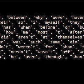
Image source : nltk_stopwords
Next question is, why should we get rid of these stopwords from our data?
These most commonly used words, which do not carry much useful information. Since it is insignificant information, we get rid of these words from our data - to focus only the words that carry more weightage.
In this case, we will not remove the negative words such as - "not", "hasn't", "wasn't" - because they actually contribute the negative sentiment of the review.

8 - Data Visualization - from the reviews
In this section we will look into the relationship between sentiment of reviews with the other factors: upvotes and downvotes. We will use bar plot [4] to depict this.
Sentiment v/s Upvotes :
As we can see in the below visualization, for the majority of the upvotes - the sentiment turned out to be positive

Sentiment v/s Downvotes :
As we can see in the below visualization, for the majority of the downvotes - the sentiment turned out to be negative

Code snippet to plot:

9 - Creating additional features from the data - for text analysis
In this step, we will create additional features such as polarity, review length and word length from the data given. This is to further analyze the data and visualize it.
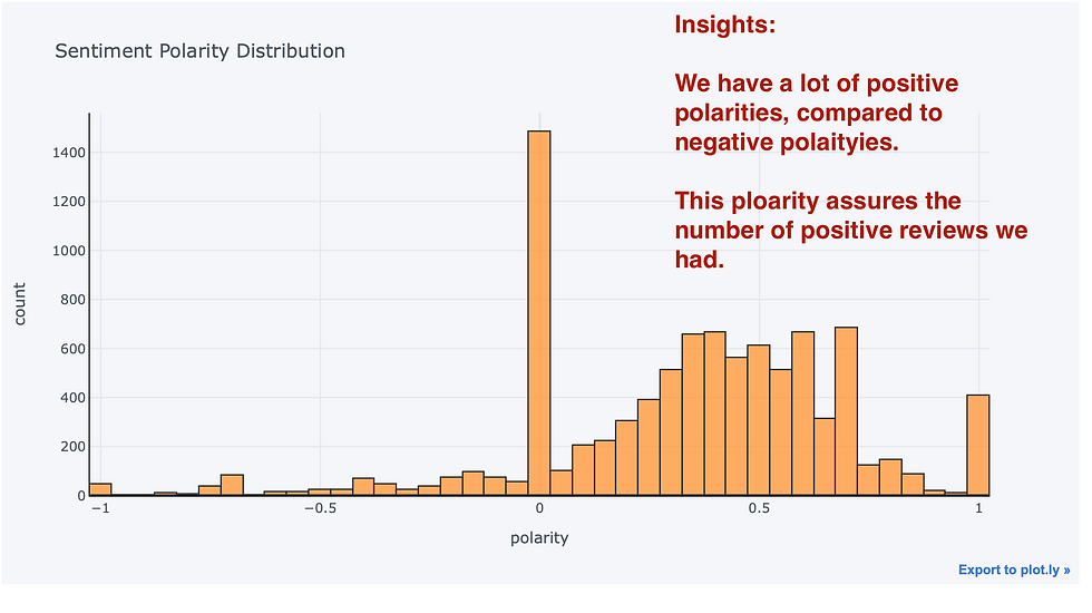
Polarity: Polarity captures how extreme the distribution of reviews are. We use Textblob for figuring out the rate of sentiment . It is between [-1,1] where -1 is negative and 1 is positive polarity [5]
Review length: Length of the review which includes each letters and spaces
Word length: This measures how many words are there in review


A - Sentiment polarity distribution
Code snippet :

Visualization :
B - Review Rating Distribution
Here, we will look into how the ratings are distributed.

C - Review Text Length Distribution

D - Review Text - Word Count Distribution

10 - Monogram, Bigram and Trigram analysis
Let's look into what this analysis does. [6]
A - First, what is an N-gram ?
N-gram means a sequence of N words
B - What kind of analysis is this?
In the given review - we will analyze how frequently a word or a sequence of words are appearing.
C - What is the significance of this analysis ?
N-Grams are useful for turning written language into data, and breaking down larger portions of search data into more meaningful segments that help to identify the root cause behind trends
D - Different kind of analysis we do:
Monogram - Here, the frequency of occurrence of a single word is measured
Bigram - considers a sequence of two words
Trigram - considers a sequence of three words.
Here we will look into Bigram and Trigram analysis - as they help us understand the words related with sentiment better.
Code snippet for Bigram analysis : (You can view the complete code my Jupyter notebook)

Below is the bigram plots for positive, negative and neutral reviews :
Here we can see, how a pair of words are related with each sentiment. And also, we can track their frequency of occurrence. This helps us give an idea on senquence of words that represent a particular sentiment.


Below is the trigram plots for positive, negative and neutral reviews :
In this plots, we can see a sequence of three words representing the sentiments.


11 - Wordcloud for each sentiment
What is a wordcloud ? [7]
A word cloud is a collection, or cluster, of words depicted in different sizes. The bigger and bolder the word appears, the more often it’s mentioned within a given text and the more important it is.
In this step, we will use this data visualization technique to see the words associated with each sentiment.
A - Wordcloud - for Positive reviews
If we observe in the below wordcloud, the words such a good, super, sound, clear etc. are reprinting the positive reviews.
Code snippet (except the variable names, it looks similar for neutral and negative reviews as well)

Visualization:

B - Wordcloud - for Neutral reviews
Our neutral reviews contains words like good, sound, bass find, well etc.

C - Wordcloud - for Negative reviews
Our negative reviews - contains the negative words like - dont't, won't, can't, paining, objective etc. - related to the products highlighted such as earphone, headphone, battery

12 - Text Normalization - Stemming v/s Lemmatization
In this step, we will normalize our text using the Stemming approach.
A - What is Stemming? [8]
Stemming is the process of converting multiple forms of the same word into one stem, to simplify the task of analyzing the processed text.
B - What is Lemmatization? [8]
Lemmatization is also used for the same purpose, for grouping together of different forms of the same word.
C - What is the difference between Stemming and Lemmatization ? [8]
Stemming uses the stem of the word
While, lemmatization uses the context in which the word is being used.

Image source : stemming_lemmatization
In our case, we will be using Stemming - as it is faster compared to lemmatization.
Extracting the reviews for processing:

Performing stemming : As we can see a sample review after stemming, the word looking has been reduced to look, purchase to purchas.

13 - TFIDF (Term Frequency - Inverse Document Frequency)
TF-IDF stands for “Term Frequency — Inverse Document Frequency”. This is a technique to quantify a word in documents, we generally compute a weight to each word which signifies the importance of the word in the document and corpus. This method is a widely used technique in Information Retrieval and Text Mining. [9]
Here we are splitting as bigram (two words) and consider their combined weight.Also we are taking only the top 5000 words from the reviews.
Also, SMOTE (Synthetic Minority Oversampling Technique) is used to balance out the imbalanced dataset problem. It aims to balance class distribution by randomly increasing minority class examples by replicating them. [10]

14 - Train-Test-Split
Now, it's time to split our data into train and test data. Using the train-test-split function dividing the data into 80:20 ratio for train and test data respectively.

15 - Building various models using different algorithms
As mentioned in the previous section of this blog, we will be using below algorithms to build various models:
1 - Logistic Regression
2 - Decision Tree
3 - KNN
4 - SVM
5- Naive Bayes
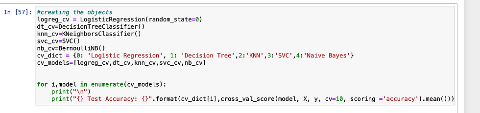
Now, let's look into the accuracy that we obtained for these models :
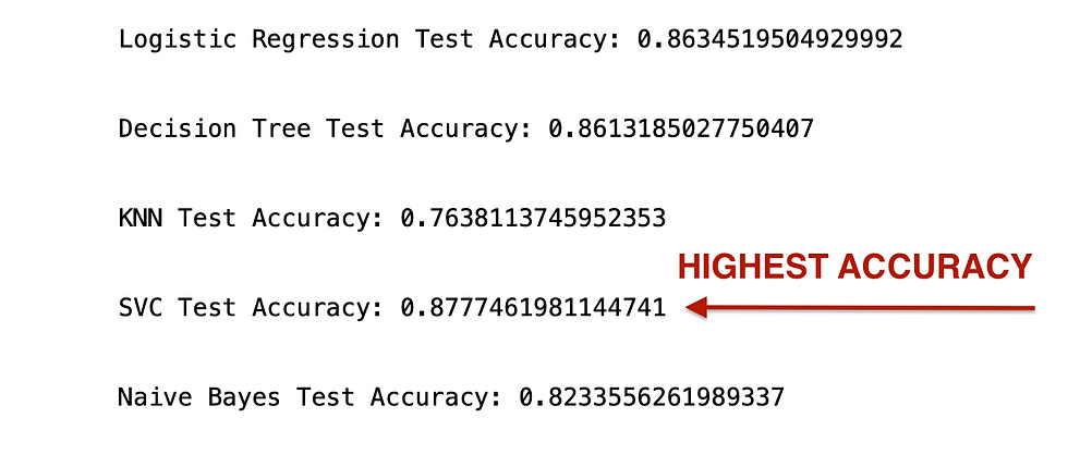
As we can see above, we've obtained the highest accuracy for SVM algorithm.
16 - Hyperparameter tuning and Experiments
In this section, I will walk you through the various experiments I conducted on this existing model. I performed the experiments with various hyper parameters, to observe and analyze the behavior of the model.
First, I picked up SVM model to perform my experiments - as we got the highest accuracy for SVM model.
A - Experiments on SVM Model :
Below screenshot depicts the Experiment 1 and 2 details. Please look into the parameters details carefully.
I'm considering different kernels such as polynomial, linear and RBF, for my experiment.
Kernel = RBF


Kernel = Polynomial

Kernel = Linear ( Observations and comparisons )
Observation : For the same set of hyper parameters - RBF Kernel performed better in comparison with Linear kernel. As seen above, RBF kernel achieved 0.86 accuracy for the same set of parameters.
Where as, Linear kernel achieved - 0.80 accuracy

Observation and very slight improvements for SVM Model :
From the above experiments, I observed that I got the a very slight increase in the accuracy by 0.01 % - over the existing model - for the below hyper parameters:
{ C= 60 , GAMMA = 2, KERNEL='RBF'}
Existing model accuracy = 0.87
My model accuracy = 0.88
Plotting Confusion matrix for the above mentioned SVM model :


Evaluation Score :

B - Experiments on Linear Regression Model :
Below screenshots, depicts my experiments on Logistic Regression model.
Observations : Please observe the below details carefully

As seen below, I obtained a 1 percent increase for my 3rd model - with hyper parameters :
C = 500 and random_state = 0.
Existing logistic regression model accuracy : 0.86
My slightly improved model accuracy : 0.87

Plotting Confusion matrix for the above mentioned Linear regression model with 0.87 accuracy :

Evaluation Score :

C - Experiments on Decision Tree Model :
For performing the experiment on the decision tree hyperparameters, I picked up two parameretes -
- criterion
- max_depth
1 - Below screenshot depicts my experiments on criterion. I observed that when criterion = gini, the accuracy was 0.83. And, when the criterion = entropy, accuracy obtained was 0.82

2 - When max_depth = None (i.e not specified)

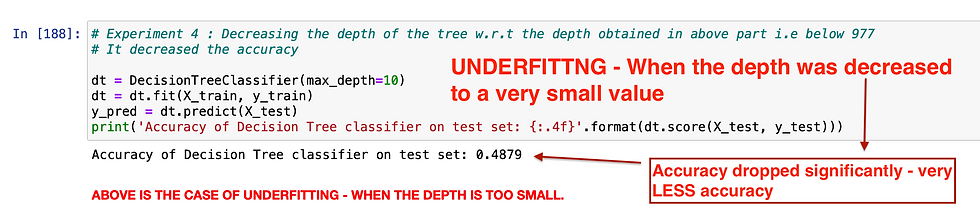
3 - Decreasing the max_depth value - caused UNDERFITTING and dropped the accuracy on test set significantly.
4 - Increasing max_depth above 977 - didn't observe much variations in the accuracy when I increased the max_depth to 2000

17 - Conclusion and Comparison :
A - Which model performed better for this dataset?
As we observed above, SVM model performed better compared to all other models.
B - What could be the reason SVM model performed better than others?
From my understanding, SVM performed better - because it uses less computation and performs better in high dimensional spaces.
C - Which kernel amongst RBF, Polynomial and Linear kernel performed better in this case?
As we observed in the above experiments - we obtained the highest accuracy with RBF Kernel, compared to linear and polynomial kernel.
D - Why KNN did not perform well on this dataset?
KNN fits good when the input data is smaller, since it's the distance based metric. In real time, it just takes lots of time to predict for the huge datasets.
Contributions :
As I have mentioned in the acknowledgement section, I followed the tutorial to get started with this implementation. I understood every piece of code and its functionality.
On top of this existing model, I performed my experiments on the different hyper parameters, for the models - SVM, Logistic Regression and Decision Tree.
As part of my experiment for SVM model, I obtained a very very slight increase in the accuracy for the hyper parameters : { C= 60 , GAMMA = 2, KERNEL='RBF'}
Existing SVM model accuracy was 0.87, and I obtained 0.88 accuracy
For Logistic Regression model, I obtained a model with 1 % increased accuracy on top of exisiting model. ( C = 500 ). Though, it's not that great of an improvement - I was at least able to arrive to slight improvement based on my experiments.
For Decision Tree model, I was able to observe the "Underfitting" scenario in my experiment - when I decreased the max_depth value to very less value (max_depth = 10 ).
Also, I experimented on the scenarios where criterion = gini AND criterion = entropy.
I hope that, after reading this blog it is pretty evident that - I took so much effort to explain each code snippet in the exisiting model - as best as I can. Along, with all the clear explanation of the concepts.
Challenges I faced and how I overcame those hurdles :
Initially when I looked into the exisiting model, it felt really overwhelming to understand each concept and code snippet that was involved in that.
It took me so much time to go through the code.
I watched multiple YouTube videos and referred multiple blogs on each concepts and prepared my own notes - to better understand that.
So that way, I was able to explain the concepts clearly in this blog.
When I started the hyper parameter tuning, GridSearchCV was taking so much time to give the results.
So I performed experiments on my own, giving the random values for hyperparameters that seemed okay for me. In this way, I was able to arrive at few observations.
References
[1] Tutorial Link:
[2] Stopwords :
[3] NLTK Stopwords :
[4] Data Visualization:
[6] N-gram analysis:
[7] WordCloud:
[8] Stemming and Lemmatization:
[9] TF-IDF:
[10] SMOTE :
[11] Logistic Regression:
[12] KNN:
[13] SVM:
[14] Decision Trees:
[15] Naive Bayes Classifier:

Comments